Layers present in Yukon2.mxd

The following data was provided by the North Yukon Planning Commission and was analysed using ESRI's ArcGIS software. Some manipulation of the layers was necessary in order to get the desired results, which will be described below. The following layers were deemed essential for our analysis:


yt_planning_regions_250k

This layer outlines the administrative divisions of the entire Yukon Territory, as shown in the image below.





nypr_lmu_mar08

This layer outlines the landscape management units (LMU) specific to the North Yukon administrative region. "LMUs are distinct areas of land that have similar ecological properties (landform and vegetation) or were previously delineated (e.g. Old Crow Flats SMA). The borders of the units are usually drawn around rivers, roads, existing SMAs or identifiable features. LMUs are intended to form the spatial framework for cumulative effects monitoring" (Metadata NYLMU, 2008). There are 13 different LMUs in the given region, as shown in the image below. For the sake of this project, measurements of landscape fragmentation will be made according to the region's 24 sub-units.





nypr_linear_features_50k

This layer shows linear features present in the North Yukon region. Linear features include: access roads (AR), main roads (MR), national roads (roads), seismic lines (SL), trails(TR) and winter roads (WR). This layer was used to measure linear density in the Eagle Plain study area as well as for the entire North Yukon Region. Buffers were not added to these features as width is not taken into consideration when measuring linear density. The image below shows these linear features along with the previous layers. The Eagle Plain study area, where the highest concentration of land use disturbance is found, is outlined in black.






ny_footprint and "footprint without buffers"

This layer is very similar to the previous layer, only that it includes all linear and non linear land use footprints. Effective mesh size measurements was based on the "footprint without buffers" layer, whereas the "ny_footprint" was used to measure surface disturbance. Further manipulation of this data will be discussed below when describing the "Union FG1" and "Union FG2" layers.

NY_LT_2005 & NY_LTRC_2005

This layers is a raster biophysical map for the NY. ''Landscape types were classified and mapped through the NY Biophysical Mapping Project using a predictive modeling approach. The NY biophysical map currently contains 18 district landscape types and 10 seral types for a total of 28 biophysical units" (NYLTRC metadata, 2005). For the purpose of setting criteria for the fragmentation geometries (FG), I initially wanted to create a layer for all water bodies. Unfortunately, given the time constraints I am limiting the analysis to two FGs. However, it may become useful if more FGs are to be included.

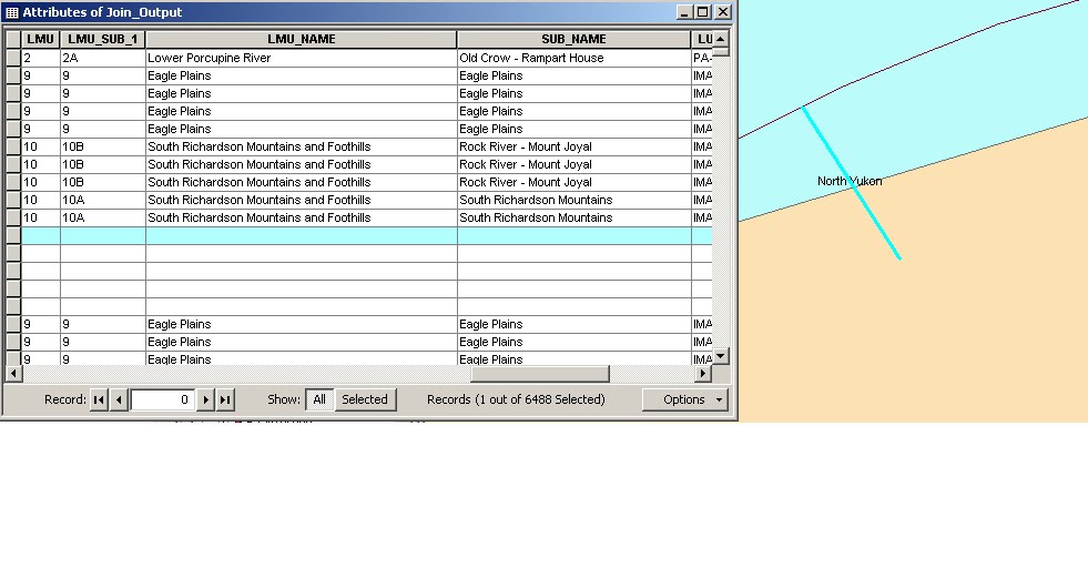
Join_Output

In order to measure linear density for both the Eagle Plain study area and the entire North Yukon Region, a spatial join was needed to join attributes from the "nypr_linear_features_50k" and the "nypr_lmu_mar08" layers. As a result, the majority of the linear features were associated with a sub unit, thus facilitating the linear density calculation. However, some features were not associated with any sub unit in the table, despite them being located within a sub unit when selected. This issue will be further discussed in a later section. (I suspect that when a linear feature crosses a sub unit boundary the table cannot compute where the feature is located since it is present in more than one sub unit. The image below shows an access road that crosses the "Rock River - Mount Joyal" and the "South Richardson Mountains" sub unit border. It will be interesting to see whether or not it is possible to cut these features along borders in order to get an accurate measurement of linear features for every sub unit. Overall, 240 individual features representing a total length of 1390.39 km were not associated with one individual sub unit. This discrepancy has no impact on the linear density calculation for the entire North Yukon Region. However, it will likely skew the results for the Eagle Plain study area as there are several features that cross over into adjacent sub units.



"Union FG1" and "Union FG2"

A union of the "nypr_lmu_mar08" and "ny_footprint" was necessary to run the effective mesh size tool effectively. In "Union FG1", all land use footprints along with the 24 sub units are present in the attributes table. "Union FG2" is similar, only seismic lines have been removed in order to measure the second FG. In both cases, sub units were given a value of 1 in the "patch" column in the attributes table, whereas disturbances were given a value of 0 (see image below).



Patch Size FG 1 (x2) and Patch Size FG 2 (x2)

These four layers are the result of running the effective mesh size tool for both fragmentation geometries. For each FGs, one of the layers displays the cross-boundary procedure (CBC) and another displays the CUT procedure. Identical value ranges were used for both FGs in order to compare differences between FGs. For both the CBC and CUT procedures, values were divided into 6 classes and colors range from red (more fragmented) to green (less fragmented). The image below is a representation of the effective mesh size (CBC) for FG 1.

FGs

In order to quantify landscape fragmentation, it is first necessary to identify which landscape elements are relevant to the ecological process or organism affected by the fragmentation (Gontier et al., 2006; Girvetz et al., 2008). The specific choice of fragmenting elements defines a so-called "fragmentation geometry". common fragmentation elements that define fragmentation geometries include, but are not limited to: roads, railroads, areas of urban development, industrial zones, and agrivultural fields (Girvetz et al., 2008). Although there is a potential for several fragmentation geometries, we have selected two for our analysis. The limited amount of literature available on the use of the effective mesh size in remote regions similar to the North Yukon has made it difficult, if not impossible, to compare our results with other studies. It is therefore important to use fragmentation geometries that are relevant to this particular study area. Large rivers and other water bodies, and high mountains may also act as barriers to animal movement and can be included in order to detect the combined barrier effect of the relevant natural and anthropogenic landscape elements(Gerlach and Musolf, 2000; Girvetz et al., 2008). Given that the area has a sub-Arctic climate, is one of the most extreme climate regions in Yukon and that continuous permafrost underlies most of the area (NYPC, 2009), potential barriers such as rivers and larger water bodies were not considered in our analysis. Also, since elevation ranges from 325 metres in Old Crow Flats to 1,800 metres in the North Ogilvie Mountains (NYPC, 2009) we have concluded that these mountain ranges were not high enough to be considered as barriers in the landscape. As a result, only the following linear and non-linear feature types present in the footprint data were taken into consideration:

Linear Features

Major Road;
Access Road;
Winter Road;
Community Use Trail;
Trail;
Seismic Line.

Non-Linear Features

Airstrip;
Well Site;
Gravel Pit;
Mine Site;
Settlement;
Traditional Camp;
Tourism / Visitor Facility.

A common distinction between these land use footprints is whether or not they are condidered permanent disturbances. Non-permanent disturbances will likely have a shorter lifespan than permanent features due to the natural re-vegetation of some feature types (NYPC, 2009), as described in the table below. The North Yukon Planning Commission (2007b) estimated that at least 20% of the non-permanent features have been re-vegetated through natural processes, with wildfire playing an important role (NYPC, 2009). Furthermore, the North Yukon Land Use Plan uses the following definition for determining when a land use disturbance, such as a seismic line, may be considered re-vegetated (reclaimed):

"a linear feature or other human-caused surface disturbance that in its current state, does not facilitate increased access or travel. In forested areas, a feature can be considered reclaimed when it contains woody vegetation (trees and / or shrubs) approximately 1.5m in height" (NYPC, 2009).



The first FG includes all land use footprints listed above. By doing so, this FG measures the overall current level of landscape fragmentation in the North Yukon Region.

Measuring Linear Density

In order to make a proper comparison between indicators (linear density, surface disturbance and effective mesh size) it was necessary to measure all features in each of the region's sub units. The "nypr_linear_features_50k layer" contained the following linear features in the landscape:

Access Roads;
Major Roads;
Roads;
Seismic Lines;
Trails;
Winter Roads.

A spatial join was required to measure the linear density (km/km2) for each sub unit. Therefore, the attributes table of the layer with the 24 sub units "nypr_lmu_mar08" was joined to the attributes table of the linear features "layer nypr_linear_features_50k". The window below shows the options that were selected to join these two tables.



The majority of the linear features are now associated with a sub unit, which will facilitate the linear density calculation. However, some features are not associated with any sub unit in the table, despite them being located within a sub unit when selected. I suspect that when a linear feature crosses a sub unit boundary the table cannot compute where the feature is located since it is present in more than one sub unit. The image below shows an access road that crosses the "Rock River - Mount Joyal" and the "South Richardson Mountains" sub unit border. It will be interesting to see whether or not it is possible to cut these features along borders in order to get an accurate measurement of linear features for every sub unit.



A table has been created for the analysis (see image below). The total length of each of the 6 linear features will need to be measured for each sub unit.

Updated project report outline

After Monday's meeting, we have agreed to modify the report's structure in order to respect the given deadline. However, the general objective of the project, which is to determine if linear density (LD) and surface disturbance (SD) are the best indicators for assessing ecological integrity, more specifically landscape fragmentation, for the North Yukon Land Use Scenarios Report, will not change. As in the initial outline, we will introduce a new indicator, the effective mesh size (meff), and will describe in detail what its advantages are over the other indicators when it comes to quantifying the ecological integrity of the region.

Assessment of the meff for the region will be slightly less detailed than anticipated. Given the timeframe, we may have to limit our analysis to two fragmentation geometries (FG). The first FG will offer a general measurement of the meff by including everything that is considered a disturbance in the landscape. The second FG will remove features that have the potential to be re-vegetated through natural processes, such as seismic lines. Our rationale behind this is that over time these features are much less significant barriers in the landscape, which may be worthy of attention of the meff is to be used in future scenario models. In addition to the meff, LD and SD will need to be measured in order to compare results between indicators. Tables with results will be created, similar to the image below:

What is the total amount of human-caused surface disturbance (SD) in each of the 24 sub units?

Results will be given in km2 of total surface disturbance per km2 of the sub unit's land cover and also the percentage of land covered by disturbances per sub unit.



A similar table will be made to show results of linear density for each of the sub units.

What is the linear density in each of the 24 sub units?

Results will be given in km per km2 of the sub unit's total land cover.

A similar table will be made to show results of the meff for both FGs. Also, a table will be made to compare results of the two meff measurements, the cross-boundary connection (CBC) and the CUT procedure.

The following sections of the report will give a detailed methodology of each step that was undertaken while manipulating the data given to us by the North Yukon Planning Commission. The purpose of this section is to give as much information as possible as to what has already been done and what the recommendations are for future analysis. Here is a brief overview of the sections:

1) Effective mesh size tool in ArcGIS
Instructions and use;
Outputs;
Current assessment of results.

2) Assessment of the NY scenarios report
Interpretation of initial data as it was received;
What needed to be done with data in order to get the desired results;
Potential questions or issues that still need to be adressed.

3) Fragmentation geometries
Possible useful combinations (recommendations);
Executed FGs.

4) Discussion and recommendations
Interpretation of the results;
Reflections on what still needs to be adressed (i.e. what's a smart path to take for someone that will carry on this project).

5) Warnings
All the issues and discrepancies encountered during this project.


Our goal is to make the transition process (from myself to the person that will pursue this project) as clear and concise as possible. Addressing what has been done and making recommendations as to how this project can be improved will hopefully help anyone who wishes to pursue this project.

Landscape fragmentation can be defined as the breaking up of a habitat, ecosystem or land-use type into smaller parcels (Forman, 1995). It is the disintegration of existing geographical patterns by the introduction of new elements or structures in such a way that the existing or desired functions are impaired (Gunlinck and Wagendorp, 2002). Ecosysem fragmentation can be described by three main effects: increase in isolation of the ecosystem patches, decrease in their size, and increase in their exposure to external disturbances, which in turn may lead to a decline in the ecosystem biodiversity as well as in its stability and ability to recover from disturbances (Geneletti, 2002; Baskent, 1999; Saunders et al., 1991). Recently, much of the literature on this topic has attempted to quantify the degree of landscape fragmentation through the use of landscape metrics and indicators. There has been a considerable effort in this field in the last two decades, enables by the rapid development of remote sensing and geographic information systems (GIS) (Herzog, 2002).

The North Yukon Planning commission released a land use scenarios report in 2009 in an effort to facilitate informed discussions about key land use issues and practices, levels of landscape change, and potential land use impacts. The project had three major objectives: 1) explore potential outcomes of plausible future land use scenarios in the North Yukon Planning Region, 2) identify and explore natural factors and human land uses and land use practices that act as key drivers of landscape change, and 3) compare the potential outcomes of different future land use scenarios against a set of socio-economic, land use and ecological indicators (NYPC, 2009). The report used two indicators, linear density and surface disturbance, to assess the levels of landscape disturbance. The former is defined as the total length of all linear features (roads, trails, pipelines, seismic lines, etc.) within a given area; it is expressed as km of linear features per km² of study area (km/km²). The latter is defined as the visible “footprint” of human land use; it is the amount of area physically disturbed by human activities. The total amount of surface disturbance is measured either in hectares (ha) or the proportion of the study area affected (%) (NYPC, 2009).

The purpose of our study is to determine if linear density and surface disturbance are the best indicators for assessing ecological integrity, more specifically landscape fragmentation, for the North Yukon Land Use Scenarios Report. This study will explore other projects that have used these indicators and will assess whether or not they were the most suitable in this particular context. Cultural interpretation and the historic dimension of the landscape are important factors in the definition of adequate references in fragmentation studies (Gunlinck and Wagendorp, 2002). Given the wide range of indicators available, the study will look at the advantages and drawbacks of linear density and surface disturbance and why they were chosen as indicators for the North Yukon Land Use Scenarios Report. In addition, this paper will introduce a third indicator, the effective mesh size (m_eff), in an effort to further analyse the degree of landscape fragmentation in the North Yukon Region. Effective mesh size is an expression of the probability that any two locations in the landscape are connected and therefore not separated by barriers such as roads (Jaeger, 2000). It can also be interpreted as the average size of the area that an animal placed randomly in the landscape will be able to access without crossing barriers (Girvetz et al., 2008).

· Discuss fragmentation geometries (FG) and differences in CUT and CBC measures

· Discuss how this may tie into existing and future scenarios reports

Working with meff tool in ArcGIS

After researching the effective mesh size tool in further detail I have discovered how exactly the original layers needed to be manipulated in order to get the desired results. I ran into some problems running the tool with buffers around features, so I decided to run it using shapefiles without buffers. To my understanding, the union tool was needed to create a new layer combining features from two different shapefiles. In this case, the "footprint without buffers" and nypr_lmu_mar08" layers were used as input features and the result was a new layer called "Union_Without_Buffers". This new layer has a column in the attributes table called patch, which codes features as 1s or 0s. Notes on the effective mesh size tool state that areas that are not covered by fragmenting elements (the suitable patches) should be coded as 1 in some field (barrier layer field). The areas covered by fragmenting elements (and their buffers) can be removed to make the shapefile smaller, however, if the fragmenting elements are left, then they should be given a value of 0 in the barrier layer field. Values in the patch column were opposite of this such that fragmenting elements were given a value of 1, whereas areas not covered by fragmenting elements were coded as 0. As a result, I simply edited the table and removed all fragmenting elements and replaced the 0 values in the 24 remaining rows (for each SU) with the value 1.

The tool ran successfully and the output file "mapunits" was created. The field "effmeshCBC" is the effective mesh size calculated using the cross-boundary connections method, while the "EffMesh" field is the effective mesh size calculated using the CUT method (as presented by Moser et al., 2007). Range of values according to each SU were mapped (see image below).



However, there seem to be inconsistencies with the results and the actual footprint data. On the one hand, the Eagle Plains Region has a high concentration of disturbances and is shown by the proper gradient, in this case blue. On the other hand, the Vuntut National Park Sub-Unit (the Northernmost SU in the North Yukon) is also represented by the same gradient, despite having very few disturbances present. Also, I am unsure as to what these values mean. This issue will need to be raised during the meeting on Monday, April 26th.

Meff

The application of effective mesh size requires specification of the landscape elements that cause fragmentation, and the definition of scales over which fragmentation is to be determined. The combination of these selections defines the fragmentation geometry (FG) (Jaeger et al., 2008). In an attempt to evaluate the suitability and reliability of meff as a landscape indicator, the following will address these questions:

• What are the advantages of using meff as an indicator of landscape fragmentation and what exactly does it measure?
• What is the extent of landscape fragmentation in the North Yukon Region today?
• what are the current values of meff in the North Yukon?
• How variable is meff among the different landscape management units (LMU) and sub-units?
• Which FG(s) is/are the most suitable one(s) to use?

The North Yukon Planning Commission has already conducted land use scenario modelling using the ALCES landscape computer simulation model to explore and better understand potential outcomes of plausible oil and gas, tourism and mining land use activities for the North Yukon Planning Region (NYLUSR, 2009). Two indicators of landscape fragmentation, linear density and surface disturbance were used in the scenario modelling (include definitions of both LD and SD). While current estimates of landscape disturbance levels are uncertain, this uncertainty does not significantly alter the land use modelling outcomes (NYLUSR, 2009).

An analysis of the effective mesh size as an indicator of landscape fragmentation will be conducted by looking at its advantages over the two previous indicators used in the model. This report will attempt to give proper reasoning as to why effective mesh size should be used as an indicator for measuring levels of landscape disturbance in subsequent land use scenario models.

Land use modelling was conducted for two study areas: 1) the entire planning region, and 2) the Eagle Plain oil and gas basin. The Eagle Plain oil and gas basin was considered to have the highest potential to incur significant levels of land use activity in the near future and was examined in greater detail (NYLUSR, 2009). Effective mesh size will be measured for all 24 sub-units, and comparison between each of them will therefore be available.

Find quote as to why it's relevant to have FGs and another that defines it. Look as Gunlinck and Wagendorp, 2002 paper (references for fragmentation analysis in the rural matrix in cultural landscapes. Landscape & Urban Planning 58).

Criteria selection for FGs

To analyse landscape fragmentation it is first necessary to specify which landscape elements are important (Jaeger et al., 2008). In this context, it is important to make the distinction between permanent and semi-permanent features. Permanent features refer to (look up permanent features definition that may be relevant for this), whereas semi-permanent features refer to features that have the ability to disappear through natural processes such as re-vegetation. As a result, the first FG will single out features whose life-span are 30 years or below (seismic liens and community use trails. Refer to table 5 on seismic lines and table 6 on estimated footprint lifespan, p. 21-22 of NYLUSR, 2009).

Using Meff Tool

After going over the instructions on how to use the effective mesh size tool in ArcGIS, I attempted to try it for myself. Here's a screenshot of the tool with the selected layers.



To my understanding, the ny_footprint layer should be put in the barrier layer field since it's the one with all the linear features. A new field (patch) was created in the attribute table. The instructions mentions that the areas that are not covered by fragmenting elements (the suitable patches) should be coded as 1 in some fields (barrier layer field). Hence, since these are all fragmenting elements, all fields were coded as 0. I'm a little confused if this layer is the appropriate one to use in this instance given that there are no features representing habitat patches, which would be represented by 1's. However, upon running the tool I noticed that the following fields all had values of 0: "AreaIntSct", "AreaMult", "AreaIntSq". As a result, I ran the tool once more with all values in the new field "patch" as 1's and a whole set of values appeared in the three fields listed above.

The nypr_lmu_mar08 layer with the different LMUs and sub-units was used as the map unit layer given that it represents the planning unit areas that will be used to calculate the effective mesh size. A new field was also created in the attributes table since a unique numerical value was needed for each different value (SUB_NAME) for the map unit field. The new field is called SUM_LMU. The output directory c:\Patrick\ was used and the resulting folder (Run Name) was called intersect. The tool ran successfully and the resulting layer "intersect" was added automatically. Buffers around all features are now shaded for this layer.

The next step is to figure out what exactly the fields in the intersect layer's attribute table mean. Upon viewing the attribute table, I noticed there were numerous blank fields. I may be wrong, but these might represent polygons resulting from the added buffers. I need to confirm if I ran the tool with the correct layers.

Also, I will need to figure out how to isolate certain features in order to create different fragmentation geometries (i.e. seismic lines).

To do:

• Do further reading on effective mesh size in order to understand how to interpret it;
• Start written report as mentionned yesterday.

Working with ArcMap

After reading the user's manual for the effective mesh size tool I tried installing it on my work station. Unfortunately, I don't have administrator rights and therefore couldn't place the effMeshArcGIS folder in the ArcGIS folder.

Instead, I attempted to create buffers around footprint types as described in table 7 (page 44 of .pdf file) of the North Yukon Planning Region's Land Use Scenarios Report so I could compare their linear density and surface disturbance results with my own. The Major Roads layer, which corresponds to the Major Road footprint type, was selected and I attempted to created a 1000 metre buffer around this linear feature, but somehow the buffer was not created. Rather than working with the individual layers created for each linear feature, I decided to work with the original layer "nypr_linear_features_50k". Buffers were then created for the following features:

• Access Roads: 500m
• Major Roads: 1000m
• Road: 500m
• Seismic Lines: 100m
• Trails: 100m
• Winter Roads: 500m

The next step was to measure the total length (in metres) of each linear feature for each LMU. However, I need to get familiar with the "Spatial Analyst" tool (I've uploaded a file "Using_ArcGIS_Spatial_Analyst_Tutorial" in Google Docs). Given that the main objective of this project is to measure the effective mesh size (or density), I think it would be wiser not to spend too much time figuring out how to measure LD and SD.

List of questions to ask NY team

I've tried to match the features present in the "ny_footprint" layer with feature types listed in "table 2: Study area land use footprints" of your scenarios report. I want to be sure that I haven't made a mistake when naming the footprint types in the layer you have sent us. Here's what I've got:

• AIRS: Airstrip
• AR: Access Road
• CAMP: ?
• FISH: ?
• GRAV: Gravel Pit
• MR: Major Road
• SET: Settlement
• SL: Seismic Line
• TOWR: ?
• TR: Trail
• TRc: ?
• VISH: ?
• WELL: Well Site
• WR: Winter Road

I still don't know which feature type corresponds to CAMP, FISH, TOWR, TRc and VISH.

The footprint layer seems to be more detailed than the linear features layer as it includes not only linear features, but also surfaces that may affect the effective mesh size (or density) of the region.

The next step(s) will be to:

• try and find a computer where I can install the effective mesh tool;
• wait for a reply from NY team about the question I sent;
• start written report while I wait for the above.

I received a quick reply from Jeff Hamm about the info I needed and could therefore create buffers for each feature in the ny_footprint layer according to the corresponding buffer widths listed in table 7 of the scenarios report. I'm still unsure if buffers need to be applied when measuring the effective mesh size and will therefore need to do further research on this subject.

Making sense of files in ArcMap

Overview

The purpose of this project is to determine whether or not linear density (LD) and surface disturbance (SD) are the best metrics for assessing ecological integrity, more specificaly landscape fragmentation, for the North Yukon Land Use Scenarios Report. Footprint data has been collected to measure the degree of fragmentation using three different scenarios: oil and gas, tourism, and mining. Our project doesn't specifically deal with these scenarios, and I will therefore abstain from going into specific detail. Rather, this project will introduce a third measure, the Effective Mesh Size (or Density), that will offer a more elaborate assessment of the degree of landscape fragmentation.

Using ArcMap

The data provided to us by the North Yukon Planning Commission was analysed using ESRI's ArcGIS software. Quite a bit of time was spent making sense of the multiple layers and upon review the following layers are deemed essential for the project:

yt_planning_regions_250k
This layer outlines the administrative divisions of the entire Yukon Territory, as shown in the image below.



nypr_lmu_mar08
This layer outlines the landscape management units (LMU) specific to the North Yukon administrative region. ''LMUs are distinct areas of land that have similar ecological properties (landform and vegetation) or were previously delineated (e.g. Old Crow Flats SMA). The borders of the units are usually drawn around rivers, roads, existing SMAs or identifiable features. LMUs are intended to form the spatial framework for cumulative effects monitoring'' (Metadata NYLMU, 2008). There are 13 different LMUs in the given region, as shown in the image below.



nypr_linear_features_50k

This layer shows linear features present in the North Yukon region. Linear features include: access roads (AR), main roads (MR), national roads (roads), seismic lines (SL), traplines (TR) and winter roads (WR). The distinction between access roads, main roads and national roads still needs to be adressed. Layers have been created for each of these features in order to manipulate them individually. The image below shows these linear features along with the previous layers.



ny_footprint
This layer is very similar to the previous layer, only that features appear to be polygons rather than polylines. Even when changing the colour of these features, they still appear as grey. It is still unclear whether or not this layer will be useful in measuring the effective mesh size (or density), but I believe it is still worthy of our attention.

NY_LT_2005 & NY_LTRC_2005
This layers is a raster biophysical map for the NY. ''Landscape types were classified and mapped through the NY Biophysical Mapping Project using a predictive modeling approach. The NY biophysical map currently contains 18 district landscape types and 10 seral types for a total of 28 biophysical units" (NYLTRC metadata, 2005). For the purpose of setting criteria for the fragmentation geometries (FG), I wanted to create a layer for all water bodies. Unfortunately, I wasn't able to do so, which is something I'll have to look into.

The next step will be to:

• Describe in detail what are the advantages of using meff when measuring landscape fragmentation in the context of cumulative impact assessment;
• Measure meff for each landscape management unit (LMU) and sub-unit (SU), giving special interest to the Eagle Plain region;
• Come up with 2-3 fragmentation geographies. Based on their scenario building models, I suggest the following FG's:
• Seismic lines: linear feature that has the potential to be re-vegetated through natural processes over time;
• Winter access roads: although not as significant as seismic lines, this FG could measure the difference between summer and winter seasons;
• Although negligible, natural features (lakes, rivers, etc.) could act as barriers. Mountains will not be included in this FG since the maximum elevation in the NY region is 1800 metres.